Visual summary of some of the core ideas of Quantum Electrodynamics. The wavepacket of a matter particle has a rotation in the complex plane. This couples with an internal rotation of the electromagnetic field, encouraging its rotation. This rotation propagates outwards in space. This EM field rotation in turn causes phase differences across other matter wavepackets, causing them to accelerate towards or away from the original particle. This is the electric force! Read on for the details.

Matter

Quantum electrodynamics describes the behaviour of electrically charged matter (e.g. electrons) and its interaction with the electromagnetic field.

Consider electrons - they are a particle that have a property called spin. In particular they are spin-1/2 particles. Spin is a somewhat mysterious property of particles that we won't go into too much here.

Anyway, spin 1/2 particles such as the electron are called fermions, and can be described with the Dirac equation.

Understanding the Dirac equation is pretty tricky however - it's a weird equation which Dirac came up with to get an equation that is first order in time (meaning it has first derivatives with respect to time, but not second or higher derivatives).

The Dirac equation is similar to a wave equation, and as you will see, particles described by the Dirac equation (e.g. electrons) have very wave-like behaviour.

Let's see some simulations of various solutions of the Dirac equation:

A wavepacket moving slowly to the right (positive momentum).

The Dirac equation is an equation for a function named \( \psi \). \(\psi\) is function of position and time coordinates: \(\psi(r, t)\). It's a function from space and time coordinates to a 4-vector of complex values. Since there are 3 space coordinates and 1 time coordinate, therefore it has signature

$$ \psi : \mathbb{R}^4 \to \mathbb{C}^4 $$ From a programmer's point of view, if you were to simulate a single particle on a grid using the Dirac equation, this means that at each grid cell you store 4 complex numbers. And each complex number is just 2 real numbers.

Let's take a look at a stationary particle, described using a stationary gaussian wavepacket. This particle has zero momentum.

A stationary particle/wavepacket.

Some important things to note about the stationary particle simulation video: In the bottom middle section, you will see some phasor arrows rotating clockwise. Phasor arrows show the complex value at a bunch of spatial points. Only the red arrows are non-zero length here: this means that \(\psi_1\) is non-zero, the other \(\psi\) components are (nearly) zero.

The top-right section shows the momentum density G, from which you can see the electron spin direction (out of the screen in this case along the +z axis). Note however that the electron spin direction is *not* correlated with the direction of rotation of the complex phasor values.

To reinforce that point, here's a video of a spin-down particle, e.g. one whose spin vector points in the -z direction (into the screen). Note that the momentum density curls in the opposite direction, but the phasor arrows rotate in the same clockwise direction as for the spin-up particle.

A stationary particle/wavepacket with spin down (-z).

Now let's look at anti-matter! These solutions are referred to as negative energy solutions:

A stationary negative energy (antimatter) particle/wavepacket

The crucial difference visible in the antimatter video above is that compared to normal matter, the phasor arrows spin in the opposite direction: anti-clockwise. Indeed, that's basically what antimatter is: it's a solution to the Dirac equation where the rotation direction in the complex plane goes the opposite direction from normal matter.

The effect of matter on the electromagnetic field

In standard quantum electrodynamics, we have a value called \( \rho \), which is the probability density of \(\psi\) at a particular position and time. For the Dirac equation, $$ \rho = \psi^\dagger \psi = |\psi_1|^2 + |\psi_2|^2 + |\psi_3|^2 + |\psi_4|^2 $$ In other words, the probability density \(\rho\) is equal to the sum of the squared lengths of the psi vectors in the complex plane.

This is what is drawn in the bottom left section of the videos above. Note that \(\rho\) is greater than or equal to zero for both the matter and antimatter particles!

The probability density \(\rho\) then affects \(\Phi\), the electric potential, in the following way (in the Lorenz gauge): $$ (\frac{1}{c^2} \frac{\partial^2}{\partial t^2} - \nabla^2) \Phi = q \rho $$ Where \(q\) is the electric charge of the particle, and has magnitude equal to the coupling constant between the dirac and EM field.

Rearranging: $$ \begin{aligned} \frac{1}{c^2} \frac{\partial^2}{\partial t^2} \Phi = q \rho + \nabla^2 \Phi \\ \frac{\partial^2}{\partial t^2} \Phi = c^2( q \rho + \nabla^2 \Phi) \end{aligned} $$ In words: the 'rate of change of the rate of change with respect to time' (the acceleration) of the electric potential \(\Phi\) is equal to \(c^2\) times the electric charge \(q\) times the probability density of the Dirac matter field (\( \rho \)) plus the 'curvature' \(\nabla^2\) of \(\Phi\).

One key point is that a blob of particle will always try to push \(\Phi\) in the direction of \(q\): That is, if \(q\) is positive, then the particle will push \(\Phi\) in the positive direction, resulting in a positive electric potential in the EM field. If \(q\) is negative, then a particle blob will push \(\Phi\) in the negative direction, resulting in a negative electric potential.

But note that \(\rho\) is always ≥ 0 for the Dirac equation, both for matter and antimatter. This means the Dirac equation cannot distinguish between the charge of a matter particle and the opposite charge of the antiparticle.

This is handled in standard QED during 'second quantisation', when QED becomes a theory of operators acting on field states, and the negative sign comes from anticommutation of fermion creation and annihilation operators.

Can we solve this issue without second quantisation? I think so! The key is to use the direction of rotation of the matter wave in the complex plane to source \(\Phi\), instead of just \(\rho = |\psi_1|^2 + |\psi_2|^2 + |\psi_3|^2 + |\psi_4|^2\), which does not contain this information. But to do this we need to abandon the Dirac equation and go back to a second-order equation of motion for the matter field.

If we square the free Dirac equation ('free' = the equation for a particle not interacting with an EM field), we get the Klein-Gordon equation (See technical appendix 'Klein-Gordon equation from the Dirac Equation').

If we square the non-free Dirac equation (e.g. square the equation for a particle interacting with an EM field), we get the Feynman-Gell-Mann equation (FGM equation)[1].

Crucially, for the Klein-Gordon equation, \(\rho\) changes to become $$ \rho = -\frac{\hbar}{m c^2}|\psi|^2 \frac{\partial (\arg \psi)}{\partial t} \\ $$ In other words, the charge density \(\rho\) is proportional to the square of the magnitude (length of phasor vectors) of \(\psi\), multiplied by the signed rate of rotation of \(\psi\) in the complex plane. (See technical appendix 'Klein-Gordon charge density and phasor rotation direction')

\(\rho\) for the 2 Klein-Gordon components that describe a Dirac-like particle becomes: $$ \rho = -\sum_{i=1}^{2} \frac{\hbar}{m c^2}|\psi_i|^2 \frac{\partial (\arg \psi_i)}{\partial t} \\ $$ i.e. we sum the individual component \(\rho\) values.

With the squared Dirac equation, a particle and an antiparticle will have opposite rotation directions in the complex plane, resulting in opposite charge densities. The value of \(q\) can have the same sign for both particle and antiparticle solutions - and the resulting opposite electrical potentials will come from the opposite directions of phase rotation!

The other nice thing about the Klein-Gordon equation is that it's much easier to understand, in my opinion, than the Dirac equation, because it isn't full of 4x4 matrices!

I plan to write another essay on understanding the Klein-Gordon equation, stay tuned for that. Many answers to the mysteries of the universe are contained within it!

With all that said, let's move on to the core intuition-building of how the Dirac matter field and the EM field interact:

The intuition for the interaction of the Matter and EM fields

In broad strokes:

1. Matter rotating in the complex plane encourages a corresponding rotation in the complex plane of the EM field.

2. This rotation in the EM field spreads outwards like a wave.

3. This rotation in the EM field in turn encourages a corresponding rotation in the matter field.

To explain this in more detail, first let me introduce the metaphor of a clutch.

The simplest kind of clutch is basically two metal discs connected to axles. When they are 'engaged' (pushed together), rotation of one of them causes, via friction, corresponding rotation in the other disc. If you have ever driven a manual car, then you will have been manually controlling a clutch. When the clutch is engaged, the engine drive shaft engages to the shaft that runs to the wheels, causing the wheels to turn.

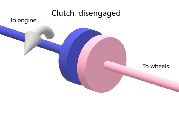
A clutch with the two clutch discs separated. The shaft from the engine does not turn the shaft to the wheels.

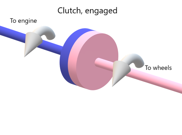
A clutch with the two clutch discs touching. Friction between the discs causes the wheel shaft to turn also.

See How a clutch works. (3D Animation) for a short introduction to clutches.

In QED, matter has a rotation in the complex plane. Some of this rotation comes from momentum, some of this rotation comes from mass. This rotation couples (engages) with the rotation of the EM field, which also can be thought of as having a rotation in the complex plane. It's not a 1:1 correspondence of rotation, indeed the matter rotation is generally much faster. It's like the clutch between the rotations is only weakly engaged. The rotation of the matter field 'encourages' rotation of the EM field.

If we identify \(\Phi\) as the rate of rotation in the complex plane of the EM field, then the equation we saw before $$ \frac{\partial^2}{\partial t^2} \Phi = c^2( q \rho + \nabla^2 \Phi) $$ Starts to make sense - it's basically saying to increase the rotation speed of the EM field if the rotation of the matter field is positive, and to decrease it if negative. Or to be a little more precise: increase the EM field rotation speed in the clockwise direction if the matter field is rotating in the clockwise direction, and to increase the EM field rotation speed in the anticlockwise direction if the matter field is rotating in the anticlockwise direction. (That is for positive \(q\). If \(q\) is negative, e.g. we are dealing with the electron and anti-electron family, then the metaphor becomes one of a reversing clutch)

Because the equation of motion for the electric potential \(\Phi\) is a wave equation, \(\Phi\) spreads outwards in space over time. In other words, the clockwise or anti-clockwise rotation spreads outwards in space, over time.

In the ideal static case, when everything has settled down and matter is not moving and the EM field has settled down, you will get a \(1/r\) potential around a point-charge. (Or around the equivalent tightly contained matter wavepacket, if such a static packet was possible!)

So around a positive point-charge, we get the result that the rotation of the EM field phase in the complex plane rotates at a rate proportional to \(1/r\) where \(r\) is the distance from the point charge.

The electromagnetic field phase around a positive point-charge. Rotation is clockwise and the rotational rate is proportional to \(1/r\).

The electromagnetic field phase around a negative point-charge. Rotation is counter-clockwise and the rotational rate is proportional to \(1/r\).

Part 3 is where it gets interesting. This is where the rotating EM field affects the matter field. It does it in the same clutch-like manner - speeding up or slowing down the matter complex-plane rotation in the direction it's rotating.

And this is where the electric (and magnetic) forces come from - because a change in speed of rotation of the matter field = a change in relative phase of parts of a wave-packet = acceleration of the particle/wave-packet in the direction of the phase gradient!.

In a little more detail: Imagine a matter particle at rest, imagined as a Gaussian wavepacket. All parts of the matter particle have the same complex phase. (See the video 'A stationary particle/wavepacket' above).

Now the rotating EM field engages (via our metaphorical clutch mechanism) with the corresponding parts of the wavepacket. Because the EM field has a faster clockwise rotation on the right (in the positive x direction), the matter particle will start having a faster phase rotation on its right, and a slower clockwise rotation on its left.

Over time, this causes the right side of the matter particle to have an advanced phase relative to the left side of the particle. In quantum mechanics, a phase gradient basically is momentum. Anything with a phase gradient, and hence with momentum, will have a corresponding velocity. In our example, the particle slowly starts to pick up a leftwards velocity.

Because the phase gradient slowly increases with time, this means the particle speed is gradually increasing with time. Thus it is undergoing acceleration, in this case to the left. We have shown the mechanism for how a charged particle is accelerated by an electric field!

A positively charged particle picks up a phase gradient and accelerates to the left in an electric potential.

Quantum electrodynamics on a lattice

I think it's helpful to introduce QED on a lattice (or what computer programmers would call a grid, or a multi-dimensional array).

Let's start with the EM field on a lattice.

Consider a space-time lattice. For our universe we would have 3 spatial dimensions and 1 time dimension.

At each lattice site (a.k.a. grid cell), we have a U(1) phase angle, call it \(\theta\).

We then have links between lattice sites. Each lattice site has an associated lattice link to the next site in the +time direction. It also has 3 associated lattice links to the next sites in the +x, +y and +z directions. Each lattice site also has links from the adjacent sites in the -time, -x, -y and -z directions.

Let the lattice spacing be \(w_t\) in the time direction - i.e. each site differs in its time coordinate from the adjacent sites by \(w_t\). Let the lattice spacing be \(w_x\) in the spatial directions, i.e. each site differs in its spatial coordinates from the adjacent sites by \(w_x\).

Our electric potential we have identified as $$ \Phi = \frac{ \partial \theta } { \partial t } $$ Where \(\theta\) is the EM field internal U(1) phase angle.

If we advance by \(w_t\) in the time direction: $$ \begin{aligned} \theta' = \theta + \frac{ \partial \theta } { \partial t } w_t \\ \theta' = \theta + \Phi w_t \\ \end{aligned} $$ So on the lattice, writing \(\theta\) as a function of the integer lattice site index coordinates: $$ \theta(x, y, z, t) = \theta(x, y, z, t-1) + \Phi(x,y,z,t-1) w_t $$ In words: as we take one step in the positive time direction on the lattice, the internal phase angle \(\theta\) increases by the electric potential \(\Phi\) multiplied by the lattice time-step \(w_t\).

We also have a value associated with each spatial lattice link. It turns out this is where the magnetic field comes from!

In addition to our electric potential \(\Phi\), we have to introduce something called the electromagnetic vector potential, call it \(\underline{A}\). It's a 3-vector: $$ \underline{A} = (A_x, A_y, A_z) $$ \(\Phi\) sits on the lattice link in the +time direction, \(A_x\) sits on the lattice link in the +x direction, \(A_y\) in the +y direction, and \(A_z\) in the +z direction.

A visualisation of the electromagnetic field on a lattice. Only the time dimension and x spatial dimension are shown; the y and z dimensions are not shown. The red phasor arrows at the lattice sites show the value of \(\theta\).

The dynamics of the EM potentials on the lattice (in Lorenz gauge and 'natural' units where \(c=1\) and \(\hbar=1\)) are $$ \frac{1}{c^2} \frac{\partial^2}{\partial t^2} \Phi = \nabla^2 \Phi + q \rho $$ as discussed earlier, and $$ \frac{1}{c^2} \frac{\partial^2}{\partial t^2} \underline{A} = \nabla^2 \underline{A} + q \underline{j} $$

\(\underline{j}\) is the matter charge current density - a vector that gives the density of flow of the matter charge in the x, y, and z directions. Its effect on \(\underline{A}\) is basically the rule that a moving electric charge creates a magnetic field.

So we have for the x component of the vector potential: $$ \frac{1}{c^2} \frac{\partial^2}{\partial t^2} A_x = \nabla^2 A_x + q j_x $$ and likewise for \(A_y\) and \(A_z\).

The equivalent lattice update rules are:

From above: $$ \theta(x, y, z, t) = \theta(x, y, z, t-1) + \Phi(x, y, z, t-1) w_t $$ Introduce some variable to keep track of our time derivatives of \(\underline{A}\) and \(\Phi\), e.g. $$ C_i(x, y, z, t) = \frac{\partial}{\partial t} A_i(x, y, z, t) $$ then $$ \begin{aligned} \Phi(x, y, z, t) = \Phi(x, y, z, t-1) + C_\Phi(x, y, z, t-1) w_t \\ A_x(x, y, z, t) = A_x(x, y, z, t-1) + C_x(x, y, z, t-1) w_t \\ A_y(x, y, z, t) = A_y(x, y, z, t-1) + C_y(x, y, z, t-1) w_t \\ A_z(x, y, z, t) = A_z(x, y, z, t-1) + C_z(x, y, z, t-1) w_t \end{aligned} $$ and $$ \begin{aligned} C_\Phi(x, y, z, t) = C_\Phi(x, y, z, t-1) + c^2(\nabla^2 \Phi + q \rho(x, y, z, t-1)) w_t \\ C_x(x, y, z, t) = C_x(x, y, z, t-1) + c^2(\nabla^2 A_x + q j_x(x, y, z, t-1) ) w_t \\ C_y(x, y, z, t) = C_y(x, y, z, t-1) + c^2(\nabla^2 A_y + q j_y(x, y, z, t-1) ) w_t \\ C_z(x, y, z, t) = C_z(x, y, z, t-1) + c^2(\nabla^2 A_z + q j_z(x, y, z, t-1) ) w_t \\ \end{aligned} $$ where \(q\) = particle charge and \(\rho\) = matter charge density.

The laplacian (sum of second derivatives, which gives something like the upwards concavity) is, using finite differences: $$ \begin{aligned} \nabla^2 \Phi = \frac{\partial^2 \Phi}{\partial x^2} + \frac{\partial^2 \Phi}{\partial y^2} + \frac{\partial^2 \Phi}{\partial z^2} = \\ \frac{1}{w_x^2}(\Phi(x+1, y, z, t-1) + \Phi(x-1, y, z, t-1) - 2 \Phi(x, y, z, t-1)) + \\ \frac{1}{w_x^2}(\Phi(x, y + 1, z, t-1) + \Phi(x, y-1, z, t-1) - 2 \Phi(x, y, z, t-1)) + \\ \frac{1}{w_x^2}(\Phi(x, y, z + 1, t-1) + \Phi(x, y, z-1, t-1) - 2 \Phi(x, y, z, t-1)) \end{aligned} $$ and likewise for \(\nabla^2 A_x\), \(\nabla^2 A_y\) and \(\nabla^2 A_z\).

So this describes how the EM field updates on the lattice, including how it is affected by a matter field (via \(\Phi\) and \(\underline{j}\)).

So the only thing left is to describe how the matter field is affected by the EM field.

I am not going to write out the Dirac equation on a lattice because it gets a bit long to write out, but it's basically what I have coded for my simulations posted above. Instead we will just stick to the maths:

The free Dirac equation (Dirac equation for a particle not in an electromagnetic field) is $$ \begin{aligned} i \hbar \frac{d}{dt} \psi = c \alpha_1 \hat{p}_1 \psi + c \alpha_2 \hat{p}_2 \psi + c \alpha_3 \hat{p}_3 \psi + \beta mc^2 \psi \end{aligned} $$ or, multiplying both sides by \(\frac{-i}{\hbar}\): $$ \begin{aligned} \frac{d}{dt} \psi = -\frac{i}{\hbar} c \alpha_1 \hat{p}_1 \psi -\frac{i}{\hbar} c \alpha_2 \hat{p}_2 \psi -\frac{i}{\hbar} c \alpha_3 \hat{p}_3 \psi -\frac{i}{\hbar} \beta mc^2 \psi \end{aligned} $$ In an EM field it becomes: $$ \begin{aligned} \frac{d}{dt} \psi = -\frac{i}{\hbar} c \alpha_1 (\hat{p}_1 - q A_1) \psi -\frac{i}{\hbar} c \alpha_2 (\hat{p}_2 - q A_2) \psi -\frac{i}{\hbar} c \alpha_3 (\hat{p}_3 - q A_3)\psi -\frac{i}{\hbar} \beta mc^2 \psi - \frac{i}{\hbar} q \Phi \psi \end{aligned} $$

The new term $$ -\frac{i}{\hbar} q \Phi \psi $$ is saying that the complex matter phase advances due to the electric potential part of the EM field, in proportion to \(\Phi\). In other words, faster EM field complex rotation results in faster matter field rotation. The negative sign is in there because the convention is that positive energy (not antimatter) matter fields rotate clockwise in the complex plane. And as we saw earlier, a positive electric potential \(\Phi\) corresponds to a clockwise rotation of the EM field phase. So there is a negative sign so that a positive \(\Phi\) will cause a rotation of the matter field in a clockwise direction, as bare multiplication by i causes a counter-clockwise rotation.

The momentum operators \( p_1 \) etc. pick up an extra term that depends on the EM vector potential \(A\): $$ -\frac{i}{\hbar} c \alpha_1 \hat{p}_1 \psi $$ becomes $$ -\frac{i}{\hbar} c \alpha_1 (\hat{p}_1 - q A_1) \psi $$ What this is saying is something like, when applying the momentum operator \(\hat{p}_1\) (which is basically taking the derivative with respect to x, then multiplying by \(-i\hbar\)), take into account the extra rotation caused by the EM vector potential that sits on the lattice link between the current cell and the adjacent cell in the +x direction.

In other words: for a matter wave moving in the +x direction, rotate the complex phase as usual as described by the free Dirac equation, but then apply an extra twist according to \(A_1\).

This is much like how we get an extra rotation when advancing the matter field in time proportional to \(\Phi\), but in the spatial instead of time directions.

Gauge Invariance

We described a phase angle \(\theta\) of the electromagnetic field earlier, and we gave an update rule for it as we advance in time. However, notice that \(\theta\) is not used anywhere else - it does not show up in the Dirac equation, and so has no direct effect on matter.

\(\theta\) is basically completely unobservable! It was just put in to help with our intuition. What does have a physical effect is the rate of change of theta, which we identified as the electric potential. As a reminder, we had: $$ \Phi = \frac{ \partial \theta } { \partial t } $$ In other words, it's the rotational speed of the clutch that matters, not its rotation angle at any particular instant. We can add any constant value to \(\theta\) and it has no physical effect - it just means the clutches at some time are rotated differently.

This is an example of a 'gauge freedom'. Actually gauge freedom goes even further: We can add a phase that is an arbitrary function of the space and time coordinates: \( f(\underline{r}, t) \).

I.e. making the replacement $$ \theta \to \theta + f(\underline{r}, t) $$ results in the replacement for the electric potential $$ \Phi \to \frac{ \partial}{ \partial t }[ \theta + f(\underline{r}, t)] = \frac{ \partial \theta}{ \partial t } + \frac{ \partial f(\underline{r}, t)}{ \partial t } = \Phi + \frac{ \partial f(\underline{r}, t)}{ \partial t } $$ If we also make the replacement $$ \underline{A} \to \underline{A} - \nabla f(\underline{r}, t) $$ in the expression for the electric field $$ \underline{E} = -\nabla \Phi - \frac{\partial \underline{A}}{\partial t} $$ The electric field is unchanged.

Making the \(\underline{A} \to \underline{A} - \nabla f(\underline{r}, t)\) replacement in the expression for the magnetic field: $$ \underline{B} = \nabla \cross \underline{A} $$ also leaves it unchanged.

The phase of the matter field \(\psi\) also has to be updated to reflect the updated \(\Phi\) and \(\underline{A}\): $$ \psi \to \exp[-i q f(\underline{r}, t) / \hbar] \psi $$ With these replacements, the physical predictions of the equations are exactly the same.

See the Gauge Invariance technical appendix for the mathematical details.

What's the point of all this? Mostly it's just to show that QED is a gauge theory, because physicists make a big deal about it!

Limitations of this intuitive approach

The approach I have taken in this article is to use a kind of semiclassical theory, where the matter and electromagnetic fields are treated as classical fields, without their field modes being quantised.

So it's not the full theory of QED, nevertheless I think it should provide valuable intuition for QED.

Some things that full QED provides an explanation for:

Pauli exclusion: the phenomenon where two spin-1/2 matter particles (such as electrons) cannot be in the same quantum state (i.e. cannot share the same position, momentum and spin).

No self-interaction: the phenomenon where a spatially 'smeared-out' charged particle does not self-repulse or self-attract via e.g. the electromagnetic field.

Both these phenomena are handled in standard QFT via the field operator structure, which depends on second-quantisation.

See my essay 'Second Quantisation - A Quantisation Too Far' for some more details.

Further Reading/Viewing

Electromagnetism as a Gauge Theory - a wonderful YouTube video from Richard Behiel that was a significant source of inspiration for the approach taken in this essay.

Technical appendix

Klein-Gordon equation from the Dirac Equation

The Dirac equation for a free particle (a particle not affected by the electromagnetic field) is $$ i \hbar \frac{\partial }{ \partial t } \psi(r, t) = \left(-i \hbar c \underline{\alpha} \cdot \underline{\nabla} + \beta m c^2 \right) \psi(r, t) $$ Following 'Quantum Theory 2015/2016' [2], since $$ \hat{p}^i = -i \hbar \frac{\partial}{\partial x^i} $$ $$ i \hbar \frac{\partial }{ \partial t } \psi(r, t) = \left(c \underline{\alpha} \cdot \underline{p} + \beta m c^2 \right) \psi(r, t) $$ Where $$ \underline{\alpha} \cdot \underline{\hat{p}} = \alpha^1\hat{p}^1 + \alpha^2\hat{p}^2 + \alpha^3\hat{p}^3 $$ Now 'square' both sides of the Dirac equation, by appyling the operators again: $$ (i \hbar \frac{\partial }{ \partial t })^2 \psi(r, t) = \left(c \underline{\alpha} \cdot \underline{p} + \beta m c^2 \right) \left(c \underline{\alpha} \cdot \underline{p} + \beta m c^2 \right) \psi(r, t) $$ so $$(- \hbar^2 \frac{\partial^2 }{ \partial t^2 }) \psi(r, t) = [ c^2 ( \alpha^1\hat{p}^1\alpha^1\hat{p}^1 + \alpha^2\hat{p}^2\alpha^2\hat{p}^2 + \alpha^3\hat{p}^3\alpha^3\hat{p}^3 + \alpha^1\hat{p}^1\alpha^2\hat{p}^2 + \alpha^2\hat{p}^2\alpha^1\hat{p}^1 + \alpha^1\hat{p}^1\alpha^3\hat{p}^3 + \alpha^3\hat{p}^3\alpha^1\hat{p}^1 + \alpha^2\hat{p}^2\alpha^3\hat{p}^3 + \alpha^3\hat{p}^3\alpha^2\hat{p}^2 ) + m c^3 ( \alpha^1\hat{p}^1 \beta + \alpha^2\hat{p}^2 \beta + \alpha^3\hat{p}^3 \beta ) + m c^3 ( \beta \alpha^1\hat{p}^1 + \beta \alpha^2\hat{p}^2 + \beta \alpha^3\hat{p}^3) + \beta^2 m^2 c^4 ] \psi $$ $$(- \hbar^2 \frac{\partial^2 }{ \partial t^2 }) \psi(r, t) = [ c^2 ( \alpha^1\hat{p}^1\alpha^1\hat{p}^1 + \alpha^2\hat{p}^2\alpha^2\hat{p}^2 + \alpha^3\hat{p}^3\alpha^3\hat{p}^3 + (\alpha^1 \alpha^2 + \alpha^2 \alpha^1)\hat{p}^1 \hat{p}^2 + (\alpha^1 \alpha^3 + \alpha^3 \alpha^1)\hat{p}^1 \hat{p}^3 + (\alpha^2 \alpha^3 + \alpha^3 \alpha^2)\hat{p}^2 \hat{p}^3 ) + m c^3 ( (\alpha^1 \beta + \beta \alpha^1)\hat{p}^1 + (\alpha^2 \beta + \beta \alpha^2)\hat{p}^2 + (\alpha^3 \beta + \beta \alpha^3)\hat{p}^3) + \beta^2 m^2 c^4 ] \psi $$ But Dirac constructed the matrices to simplify and cancel in particular ways: $$ (\alpha^1)^2 = (\alpha^2)^2 = (\alpha^3)^2 = \beta^2 = 1 $$ and $$ \alpha^i \alpha^j + \alpha^j \alpha^i = 0 \qquad i \neq j $$ and $$ \alpha^i \beta + \beta \alpha^i = 0 $$ so $$(- \hbar^2 \frac{\partial^2 }{ \partial t^2 }) \psi(r, t) = [ c^2 ( (\hat{p}^1)^2 + (\hat{p}^2)^2 + (\hat{p}^3)^2 + (0)\hat{p}^1 \hat{p}^2 + (0)\hat{p}^1 \hat{p}^3 + (0)\hat{p}^2 \hat{p}^3 ) + m c^3 ( (0)\hat{p}^1 + (0)\hat{p}^2 + (0)\hat{p}^3) + m^2 c^4 ] \psi $$ $$ -\hbar^2 \frac{\partial^2 }{ \partial t^2 } \psi(r, t) = [ c^2 ( (\hat{p}^1)^2 + (\hat{p}^2)^2 + (\hat{p}^3)^2) + m^2 c^4 ] \psi $$ $$ -\hbar^2 \frac{\partial^2 }{ \partial t^2 } \psi(r, t) = [ c^2 \hat{\underline{p}}^2 + m^2 c^4 ] \psi(r, t) $$ $$ 0 = [ \hbar^2 \frac{\partial^2 }{ \partial t^2 } + c^2 \hat{\underline{p}}^2 + m^2 c^4 ] \psi(r, t) $$ $$ 0 = [ \hbar^2 \frac{\partial^2 }{ \partial t^2 } - \hbar^2 c^2 \nabla^2 + m^2 c^4 ] \psi(r, t) $$ Dividing by \( \hbar^2 c^2 \): $$ 0 = [ \frac{1}{c^2} \frac{\partial^2 }{\partial t^2 } - \nabla^2 + \frac{m^2 c^2}{\hbar^2} ] \psi(r, t) $$ Which is the Klein-Gordon equation.

This equality is true for each component of \(\psi\) separately: e.g.

$$ 0 = [ \frac{1}{c^2} \frac{\partial^2 }{\partial t^2 } - \nabla^2 + \frac{m^2 c^2}{\hbar^2} ] \psi_i(r, t) $$

What we have shown is that any \(\psi\) that satisfies the Dirac equation, in turn satisfies component-wise the Klein-Gordon equation, i.e. each \(\psi_i\) satisfies the Klein-Gordon equation.

Note however that not all sets of 4 individual \(\psi_i\) wavefunctions that satisfy the KG equation satisfy the Dirac equation.

Klein-Gordon charge density and phasor rotation direction

Ok now consider the 'probability density' (actually charge density) for the K.G. equation: $$ \rho = \frac{i \hbar}{2 m c^2}(\psi^* \frac{\partial \psi}{\partial t} - \psi \frac{\partial \psi^*}{\partial t}) $$ Consider psi in polar form: $$ \psi = R e^{i \theta} $$ where \(R = |\psi|\) and \(\theta = \arg \psi \)

Then $$ \begin{aligned} \frac{\partial \psi}{\partial t} = \frac{\partial R e^{i \theta}}{\partial t} \\ = \dot{R} e^{i \theta} + R \frac{\partial e^{i \theta}}{\partial t} \\ = \dot{R} e^{i \theta} + R i \dot{\theta} e^{i \theta} \\ = e^{i \theta}(\dot{R} + R i \dot{\theta}) \end{aligned} $$ and similarly $$ \begin{aligned} \frac{\partial \psi^*}{\partial t} = \frac{\partial R e^{-i \theta}}{\partial t} \\ = \dot{R} e^{-i \theta} + R \frac{\partial e^{-i \theta}}{\partial t} \\ = \dot{R} e^{-i \theta} - R i \dot{\theta} e^{-i \theta} \\ = e^{-i \theta}(\dot{R} - R i \dot{\theta}) \end{aligned} $$ so $$ \begin{aligned} \rho = \frac{i \hbar}{2 m c^2}(\psi^* \frac{\partial \psi}{\partial t} - \psi \frac{\partial \psi^*}{\partial t}) \\ = \frac{i \hbar}{2 m c^2}[ (R e^{-i \theta}) (e^{i \theta}(\dot{R} + R i \dot{\theta})) - (R e^{i \theta}) (e^{-i \theta}(\dot{R} - R i \dot{\theta}) )] \\ = \frac{i \hbar}{2 m c^2}[ R (\dot{R} + R i \dot{\theta}) - R (\dot{R} - R i \dot{\theta}) ] \\ = \frac{i \hbar}{2 m c^2}[ R ( \dot{R} + R i \dot{\theta} - \dot{R} + R i \dot{\theta} )] \\ = \frac{i \hbar}{2 m c^2}[ R ( 2 R i \dot{\theta} )] \\ = \frac{i \hbar}{m c^2}R^2 i \dot{\theta} \\ = -\frac{\hbar}{m c^2}R^2 \dot{\theta} \\ \rho = -\frac{\hbar}{m c^2}|\psi|^2 \frac{\partial (\arg \psi)}{\partial t} \\ \end{aligned} $$ So in other words, this means the charge density \(\rho\) is proportional to the square of the magnitude of \(\psi\), multiplied by the rate of rotation of \(\psi\) in the complex plane.

(Note that \(\frac{\partial (\arg \psi)}{\partial t}\) is positive for counter-clockwise rotations, but the negative sign out the front makes \(\rho\) positive for clockwise rotations)

A particle and an antiparticle will have opposite rotation directions in the complex plane, resulting in opposite charge densities.

Gauge Invariance

Making the replacement $$ \theta \to \theta + f(\underline{r}, t) $$ results in the replacement for the electric potential $$ \Phi \to \frac{ \partial}{ \partial t }[ \theta + f(\underline{r}, t)] = \frac{ \partial \theta}{ \partial t } + \frac{ \partial f(\underline{r}, t)}{ \partial t } = \Phi + \frac{ \partial f(\underline{r}, t)}{ \partial t } $$ If we also make the replacement $$ \underline{A} \to \underline{A} - \nabla f(\underline{r}, t) $$ in the expression for the electric field $$ \underline{E} = -\nabla \Phi - \frac{\partial \underline{A}}{\partial t} $$ we get $$ \begin{aligned} \underline{E} = -\nabla \Phi - \frac{\partial \underline{A}}{\partial t} = -\nabla(\Phi + \frac{ \partial f(\underline{r}, t)}{ \partial t }) - \frac{ \partial}{ \partial t }[\underline{A} - \nabla f(\underline{r}, t)] \\ \underline{E} = -\nabla \Phi - \nabla \frac{ \partial f(\underline{r}, t)}{ \partial t } - \frac{\partial \underline{A}}{\partial t} + \frac{\partial }{\partial t} [\nabla f(\underline{r}, t)] \\ \underline{E} = -\nabla \Phi - \frac{\partial \underline{A}}{\partial t} - \nabla \frac{ \partial f(\underline{r}, t)}{ \partial t } + \frac{\partial }{\partial t} [\nabla f(\underline{r}, t)] \\ \end{aligned} $$ And because partial derivatives commute (e.g. you can swap the order of \(\nabla\) and \(\frac{\partial}{\partial t}\), the last two terms cancel out, and you are left with $$ \underline{E} = -\nabla \Phi - \frac{\partial \underline{A}}{\partial t} $$ which is the original expression for \(\underline{E}\).

In the expression for the magnetic field: $$ \underline{B} = \nabla \cross \underline{A} $$ Making the same replacement $$ \underline{A} \to \underline{A} - \nabla f(\underline{r}, t) $$ gives $$ \begin{aligned} \underline{B} = \nabla \cross (\underline{A} - \nabla f(\underline{r}, t)) \\ = \nabla \cross \underline{A} - \nabla \cross \nabla f(\underline{r}, t) \end{aligned} $$ But the curl of a gradient is zero, so \(\nabla \cross \nabla f(\underline{r}, t) = 0\), and so $$ \begin{aligned} \underline{B} = \nabla \cross (\underline{A} - \nabla f(\underline{r}, t)) \\ = \nabla \cross \underline{A} - 0 \\ = \nabla \cross \underline{A} \end{aligned} $$ Which is the original expression for \(\underline{B}\).

The phase of the matter field \(\psi\) also has to be updated to reflect the updated \(\Phi\) and \(\underline{A}\): $$ \psi \to \exp[-i q f(\underline{r}, t) / \hbar] \psi $$

Let $$ R = \exp[-i q f(\underline{r}, t) / \hbar] $$ i.e. $$ \psi \to R \psi $$ And with our EM potential replacements: $$ \underline{A} \to \underline{A} - \nabla f(\underline{r}, t) $$ which becomes, component-wise: $$ A_i \to A_i - \frac{\partial f(\underline{r}, t)}{\partial x_i } $$ and $$ \Phi \to \Phi + \frac{ \partial f(\underline{r}, t)}{ \partial t } $$ Make these replacements in the Dirac eqn: $$ \begin{aligned} \frac{d}{dt}( R \psi) = -\frac{i}{\hbar} c \alpha_1 (\hat{p}_1 - q (A_1 - \frac{\partial}{\partial x} f(\underline{r}, t))) R\psi -\frac{i}{\hbar} c \alpha_2 (\hat{p}_2 - q (A_2 - \frac{\partial}{\partial y} f(\underline{r}, t))) R\psi -\frac{i}{\hbar} c \alpha_3 (\hat{p}_3 - q (A_3 - \frac{\partial}{\partial z} f(\underline{r}, t))) R \psi -\frac{i}{\hbar} \beta mc^2 R \psi - \frac{i}{\hbar} q (\Phi + \dot{f}(\underline{r}, t)) R \psi \\ -i q / \hbar \dot{f}(\underline{r}, t) R \psi + R \frac{d}{dt} \psi = -\frac{i}{\hbar} c \alpha_1 (\hat{p}_1 - q (A_1 - \frac{\partial}{\partial x} f(\underline{r}, t))) R \psi -\frac{i}{\hbar} c \alpha_2 (\hat{p}_2 - q (A_2 - \frac{\partial}{\partial y} f(\underline{r}, t))) R \psi -\frac{i}{\hbar} c \alpha_3 (\hat{p}_3 - q (A_3 - \frac{\partial}{\partial z} f(\underline{r}, t))) R \psi -\frac{i}{\hbar} \beta mc^2 R \psi - \frac{i}{\hbar} q (\Phi + \dot{f}(\underline{r}, t)) R \psi \\ -i q / \hbar \dot{f}(\underline{r}, t) R \psi + R \frac{d}{dt} \psi = -\frac{i}{\hbar} c \alpha_1 (\hat{p}_1 - q A_1 + q \frac{\partial}{\partial x} f(\underline{r}, t))) R \psi -\frac{i}{\hbar} c \alpha_2 (\hat{p}_2 - q A_2 + q \frac{\partial}{\partial y} f(\underline{r}, t))) R \psi -\frac{i}{\hbar} c \alpha_3 (\hat{p}_3 - q A_3 + q \frac{\partial}{\partial z} f(\underline{r}, t))) R \psi -\frac{i}{\hbar} \beta mc^2 R \psi - \frac{i}{\hbar} q (\Phi + \dot{f}(\underline{r}, t)) R \psi \\ -i q / \hbar \dot{f}(\underline{r}, t) R \psi + R \frac{d}{dt} \psi = -\frac{i}{\hbar} c \alpha_1 (\hat{p}_1 - q A_1 + q \frac{\partial}{\partial x} f(\underline{r}, t))) R \psi -\frac{i}{\hbar} c \alpha_2 (\hat{p}_2 - q A_2 + q \frac{\partial}{\partial y} f(\underline{r}, t))) R \psi -\frac{i}{\hbar} c \alpha_3 (\hat{p}_3 - q A_3 + q \frac{\partial}{\partial z} f(\underline{r}, t))) R \psi -\frac{i}{\hbar} \beta mc^2 R \psi - \frac{i}{\hbar} q \Phi R \psi - \frac{i}{\hbar} q \dot{f}(\underline{r}, t)) R \psi \\ \end{aligned} $$ First and last terms cancel from each side: $$ \begin{aligned} R \frac{d}{dt} \psi = -\frac{i}{\hbar} c \alpha_1 (\hat{p}_1 - q A_1 + q \frac{\partial}{\partial x} f(\underline{r}, t))) R \psi -\frac{i}{\hbar} c \alpha_2 (\hat{p}_2 - q A_2 + q \frac{\partial}{\partial y} f(\underline{r}, t))) R \psi -\frac{i}{\hbar} c \alpha_3 (\hat{p}_3 - q A_3 + q \frac{\partial}{\partial z} f(\underline{r}, t))) R \psi -\frac{i}{\hbar} \beta mc^2 R \psi - \frac{i}{\hbar} q \Phi R \psi \\ \end{aligned} $$ Consider the term $$ \begin{aligned} -\frac{i}{\hbar} c \alpha_1 (\hat{p}_1 - q A_1 + q \frac{\partial}{\partial x} f(\underline{r}, t)) R \psi \\ = -\frac{i}{\hbar} c \alpha_1 (\hat{p}_1 - q A_1) R \psi - \frac{i}{\hbar} c \alpha_1 q \frac{\partial}{\partial x} f(\underline{r}, t) R \psi \\ = -\frac{i}{\hbar} c \alpha_1 (\hat{p}_1 R - q A_1 R)\psi - \frac{i}{\hbar} c \alpha_1 q \frac{\partial}{\partial x} f(\underline{r}, t) R \psi \\ \end{aligned} $$ But $$ \begin{aligned} \hat{p}_1 R \psi = -i \hbar \frac{\partial}{\partial x} (R \psi) \\ = -i \hbar [\frac{\partial R}{\partial x} \psi + R \frac{\partial}{\partial x}\psi ] \\ = -i \hbar [\frac{\partial \exp[-i q f(\underline{r}, t) / \hbar]}{\partial x} \psi + R \frac{\partial}{\partial x}\psi ] \\ = -i \hbar [-i q / \hbar \frac{\partial f(\underline{r}, t)}{\partial x} R \psi + R \frac{\partial}{\partial x}\psi ] \\ = -i (-i) q \frac{\partial f(\underline{r}, t)}{\partial x} R \psi - i \hbar R \frac{\partial}{\partial x}\psi \\ = -i (-i) q \frac{\partial f(\underline{r}, t)}{\partial x} R \psi - R i \hbar \frac{\partial}{\partial x}\psi \\ = - q \frac{\partial f(\underline{r}, t)}{\partial x} R \psi + R \hat{p}_1 \psi \\ \end{aligned} $$ So the term becomes $$ \begin{aligned} -\frac{i}{\hbar} c \alpha_1 (\hat{p}_1 R - q A_1 R)\psi - \frac{i}{\hbar} c \alpha_1 q \frac{\partial}{\partial x} f(\underline{r}, t) R \psi \\ = -\frac{i}{\hbar} c \alpha_1 \hat{p}_1 R \psi + \frac{i}{\hbar} c \alpha_1 q A_1 R \psi - \frac{i}{\hbar} c \alpha_1 q \frac{\partial}{\partial x} f(\underline{r}, t) R \psi \\ = -\frac{i}{\hbar} c \alpha_1 [- q \frac{\partial f(\underline{r}, t)}{\partial x} R \psi + R \hat{p}_1 \psi] + \frac{i}{\hbar} c \alpha_1 q A_1 R \psi - \frac{i}{\hbar} c \alpha_1 q \frac{\partial}{\partial x} f(\underline{r}, t) R \psi \\ = -\frac{i}{\hbar} c \alpha_1 [- q \frac{\partial f(\underline{r}, t)}{\partial x} R \psi] + -\frac{i}{\hbar} c \alpha_1 [R \hat{p}_1 \psi] + \frac{i}{\hbar} c \alpha_1 q A_1 R \psi - \frac{i}{\hbar} c \alpha_1 q \frac{\partial}{\partial x} f(\underline{r}, t) R \psi \\ = \frac{i}{\hbar} c \alpha_1 q \frac{\partial f(\underline{r}, t)}{\partial x} R \psi + -\frac{i}{\hbar} c \alpha_1 [R \hat{p}_1 \psi] + \frac{i}{\hbar} c \alpha_1 q A_1 R \psi - \frac{i}{\hbar} c \alpha_1 q \frac{\partial}{\partial x} f(\underline{r}, t) R \psi \\ = -\frac{i}{\hbar} c \alpha_1 R \hat{p}_1 \psi + \frac{i}{\hbar} c \alpha_1 q A_1 R \psi \\ = -\frac{i}{\hbar} c \alpha_1 R \hat{p}_1 \psi + \frac{i}{\hbar} c \alpha_1 R q A_1 \psi \\ = -\frac{i}{\hbar} c \alpha_1 R ( \hat{p}_1 - q A_1) \psi \\ = R(-\frac{i}{\hbar} c \alpha_1 ( \hat{p}_1 - q A_1) ) \psi \\ \end{aligned} $$ Likewise for the other \(A_2\) and \(A_3\) terms.

So going back to our Dirac equation with replacements: $$ \begin{aligned} R \frac{d}{dt} \psi = -\frac{i}{\hbar} c \alpha_1 (\hat{p}_1 - q A_1 + q \frac{\partial}{\partial x} f(\underline{r}, t)) R \psi -\frac{i}{\hbar} c \alpha_2 (\hat{p}_2 - q A_2 + q \frac{\partial}{\partial y} f(\underline{r}, t)) R \psi -\frac{i}{\hbar} c \alpha_3 (\hat{p}_3 - q A_3 + q \frac{\partial}{\partial z} f(\underline{r}, t)) R \psi -\frac{i}{\hbar} \beta mc^2 R \psi - \frac{i}{\hbar} q \Phi R \psi \\ R \frac{d}{dt} \psi = - R(\frac{i}{\hbar} c \alpha_1 (\hat{p}_1 - q A_1)) \psi - R(\frac{i}{\hbar} c \alpha_2 (\hat{p}_2 - q A_2)) \psi - R(\frac{i}{\hbar} c \alpha_3 (\hat{p}_3 - q A_3)) \psi -R \frac{i}{\hbar} \beta mc^2 \psi - R \frac{i}{\hbar} q \Phi \psi \\ \end{aligned} $$ And we can cancel out R from both sides, leaving us with the original Dirac eqn without replacements: $$ \begin{aligned} \frac{d}{dt} \psi = -\frac{i}{\hbar} c \alpha_1 (\hat{p}_1 - q A_1) \psi -\frac{i}{\hbar} c \alpha_2 (\hat{p}_2 - q A_2) \psi -\frac{i}{\hbar} c \alpha_3 (\hat{p}_3 - q A_3) \psi - \frac{i}{\hbar} \beta mc^2 \psi - \frac{i}{\hbar} q \Phi \psi \\ \end{aligned} $$ Thus showing that our gauge replacements leave the physics exactly unchanged.

References

1. Theory of the Fermi Interaction, R. P. Feynman and M. Gell-Mann. Physical Review volume 109, 1957.

2. Quantum Theory 2015/2016 - Course notes from a course on quantum and quantum field theory. Author unknown.